Trying To Get A Good One

Trying to get a Good One

A story on history of crime in UK during XX century

UK is spearheading the open data movement for a couple of years now. https://data.gov.uk/ is now a repository of 20000+ datasets covering fields like Health, Education, Government spending etc. David Cameron started the wave with public letter to every government department which recommends openness with following start:

Greater transparency across Government is at the heart of our shared commitment to enable the public to hold politicians and public bodies to account; to reduce the deficit and deliver better value for money in public spending; and to realize significant economic benefits by enabling businesses and non-profit organizations to build innovative applications and websites using public data.

Pretty awesome.

For today I will play with the dataset called Summary of recorded crime data from 1898 to 2001/02. Data contains historical records on recorded crime throughout XX century grouped by categories such as homicide, harassment or a bit less gloomy ones such as theft of pedal cycle.

This is the list of crime categories in the dataset.

The weapon of choice is again going to be Python.

crimes_df = pd.read_csv('C:\\rec-crime-1898-2002.csv')

crimes_df_numeric = crimes_df.set_index(['Year']).apply(pd.to_numeric, errors='Ignore')

Additional technical notes for the brave

Before we start we need to do one more thing. In the source CSV file (coma separated file which is a simple text file with tabular data separated by column character) some of the rows contain values like ‘-’ or 'N\A' or ‘Not Available’. These inconsistencies lead to python and libraries (pandas) which I am using fail to determine the type of such columns. The type of column means for example that column contains numbers or raw text and different operations can be applied on different types. E.g. you can't calculate an average of raw text column but you can on a column of number type. Lastly we want to set index to year column. This means that every return cell will be identified by the year instead of using the row number. This may sound a bit overwhelming. I recommend following this tutorial which will give you all understanding that you need.

Another big point is that such barriers may be a showstopper for majority of people without strong programming background. I think that the bar can be lowered for majority of investigations by still keeping the freedom that raw data exploration offers.

I randomly picked ‘Attempted murder’ category just to see what the data looks like.

crimes_df_numeric['Attempted murder'].plot()
plt.title('History of attempted murder')
plt.ylabel('Number of attempted murders')

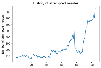
Immediately we have something interesting. We can see that crime rate fell substantially during Thatcher era and then again skyrocketed during the nineties. Year 1939 is missing (and it is also missing for other categories, not sure why). Also we can see that during WW1 there was a drop and in late WW2 there was an rise until 1950. I will leave Thatcherism for some other time and concentrate on impact of WWs on crime rate.

Let us try to find which categories went through the greatest shift during the wartimes. We will start with WW1.

There are many ways to identify changes in a time series. I will not be too sophisticated here. Instead, let us just calculate mean for every crime category during the war years ([1914-1919]) and the mean of years around the WW1 ([1910-1913) and [1920-1922]). Then we will simply subtract these numbers for every crime category. If end result is positive that means that there was an increase and if it is negative there was a decline. This is not a proper way to do this but we are not dealing with too many categories so we can afford to go manually through the most dominant ones.

around_war_years = list(range(1910,1914)) + list(range(1920, 1923))
war_years = list(range(1914,1920))

mean_difference = ((crimes_df_numeric.loc[war_years].mean() - crimes_df_numeric.loc[around_war_years].mean()).sort_values(ascending=False).dropna())
plt.title('Crime change durign ww1')
mean_difference.plot(kind='bar')

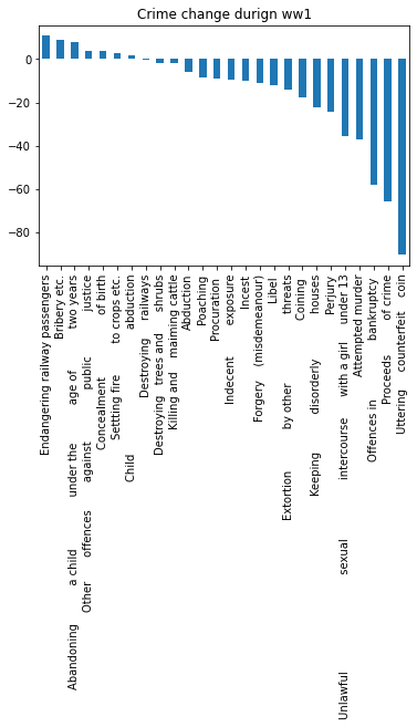
Interestingly we can see that a majority of crimes experienced a drop. The one that went through the strongest increase is bigamy! I definitely didn’t expect that. Riot is somewhat expected. Procuring illegal abortion is just one of those sad indicators on how desperate times affect common people. Same goes for abandoning a child under two.

On the right we can see that heavy crimes decreased. This may be due to sudden patriotic feeling, heavier punishments and more strict war laws, majority of male population being on the front, less accurate statistic or something else.

But come on, bigamy, really? Let us explore that in more details.

crimes_df_numeric['Bigamy'].plot()

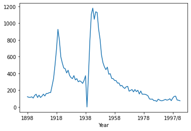
Just wow. So during the both wars bigamy in UK just exploded. I did some googling and it turns out that this is a known phenomenon. This paper (from which I shamelessly stole the title. The story goes that one gentleman who was brought to court for bigamy when asked why he had taken two wives had said it was because I was trying to get a good one.) covers in great details the history of bigamy in England and Wales. The gist is that women-men ratio changed due to war which was a great opportunity for any bigamist. Additionally on the front in France many Englishmen started relationships with French women, especially hospital nurses. French girls, as good Catholics, didn’t want to pursue sexual endeavors without proper marriage. Following this line of thought bigamy seemed to be the answer. Also statistically speaking bigamy is a pretty good approach in finding the true love.

Let us see what other interesting data we can find.

crimes_df_numeric['Procuring illegal abortion'].plot()

The increase during WW1 isn’t so dominant. But look at WW2. The London Blitz really made people desperate. Interesting is an increase in the sixties. The abortion was legalized in 1967 and you can see the drop.

crimes_df_numeric['Abandoning a child under the age of two years'].plot()

Sad. Increase during the both wars. Increase in 1990+ is scary. Good topic for some of future investigations.

I will leave WW2 for some other time. Just for an appetizer here is the mean difference between WW2 years vs. surrounding years. Looks fun 😃